AI Computational Fluid Dynamics in Medical Devices: What Has Shipped, What Is Coming, and What Cannot Work

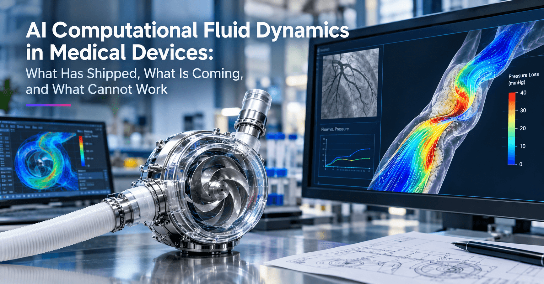
Designing a heart pump that doesn't shred red blood cells, and computing how much pressure a patient's coronary artery is losing, look like two separate engineering problems. They are the same equation, written down nearly two centuries ago. What kept both of them hard was never the mathematics — it was the clock.

1. The Navier–Stokes equations work. They are just too slow.

The Navier–Stokes equations describe where a fluid goes, how fast, and at what pressure. In principle they answer almost any flow question you can pose.

The engineering method for solving them is computational fluid dynamics (CFD) — slice the flow field into several million cells and iterate cell by cell. Denser mesh, more accurate answer, longer wait.

1.1 The equations solve. The iteration cycle is measured in weeks.

A single high-fidelity simulation runs for hours to days. Add mesh regeneration and manual post-processing, and one design iteration typically takes weeks.

1.2 What the slowness costs

Two things.

The first is R&D iteration. Change one blade angle in a blood pump and the entire mesh is rebuilt, the simulation rerun. The number of design variants an engineer can validate in a week is a limited double digit — and that number does not govern accuracy. It governs how much of the design space ever gets explored.

The second is the clinic. Intraprocedural decisions need answers in seconds to minutes. A simulation measured in hours never makes it through the cath lab door.

2. PINNs and neural operators: what AI actually changes

Start with what AI does not do here. It does not replace the Navier–Stokes equations. It replaces solving them from scratch every single time.

The approach is called a surrogate model: train a fast model on a small number of full-order simulations, then let it predict directly on new problems — trading a slice of accuracy for the elimination of almost all of the time.

Two technical branches have emerged.

2.1 PINNs: writing conservation laws into the loss function

Physics-informed neural networks (PINNs) treat the equation residual — how badly a given prediction violates Navier–Stokes — as part of the training loss. The network is optimized not only to fit data but simultaneously to suppress physical violations.

2.2 Neural operators: learning the geometry-to-flow-field map itself

Neural operators go a step further. What they learn is not the solution to one problem, but the mapping from input geometry to output flow field. Change the vessel shape, change the pump housing — no retraining required.

2.3 How much faster, actually

This is where numbers get inflated most often. The ranges that hold up are these:

Same technique, three rows, four orders of magnitude between top and bottom. The variable is not the model. It is the problem.

⚠️ Watch Out: "hundreds of times faster" circulates widely in this field, but a speedup divorced from its scenario means nothing. In turbulent, shock-dominated, strongly nonlinear regimes the return from a surrogate model drops to roughly one order of magnitude. Still worth deploying — just not the number in the marketing deck.

The same pattern has already landed on the imaging side: deep-learning image reconstruction in CT and MRI swaps iterative reconstruction for learned reconstruction — same logic, replacing physical computation with model inference.

3. Blood pump design: this is where verifiable gains exist

Inside LVADs (left ventricular assist devices) and ECMO circuits, pump design has to balance two objectives that pull against each other.

3.1 Two problems that must be solved at once

A stagnation zone is where flow velocity approaches zero. Blood sits there and tends to clot.

Wall shear stress is the frictional force the fluid exerts on the wall. Past a threshold it tears red blood cells apart — hemolysis, quantified in engineering by the Normalized Index of Hemolysis (NIH).

The difficulty is that suppressing one tends to raise the other: narrowing the flow channel eliminates stagnation but pushes shear stress up.

3.2 The verifiable numbers

Figures from a single CAD/CFD optimization study (Okamoto et al.) ⁴.

One clarification matters here: these numbers are not an AI surrogate model's record. They come from CAD/CFD optimization itself — what they show is how much headroom exists in this class of problem. The surrogate model's contribution is pushing that search from "a handful of variants per week" toward "thousands to tens of thousands of variants in hours."

4. Targeted drug delivery and microfluidics: value and boundary of patient-specific geometry

4.1 What patient-specific geometry can do

Inhaled drug delivery — asthma, targeted pulmonary antibodies — requires particles to deposit at a specific bronchial segment. The method: reconstruct the airway from the patient's CT, run a CFD particle-deposition simulation, and back out the particle diameter and inhaler geometry. ⁵

What works today: CT resolves roughly 6–12 generations of bronchi, covering the central airways.

4.2 What it cannot do

Distal small airways remain out of reach — CT resolution runs out before you get there. A single simulation still takes hours to days, and that time cost is precisely what AI surrogate models are aimed at.

Microfluidics and organ-on-chip have quantifiable progress of their own: the AI-CMDA platform compressed the design-fabricate-test cycle from weeks to under 24 hours ⁶. Most of this is still research stage, not commercial product.

5. FFR-CT: the only one that has actually commercialized

If one thing on this list has shipped, it is this.

Fractional flow reserve (FFR) has traditionally required a pressure wire. FFR-CT takes a different route: use the coronary CT angiography (CCTA) dataset to compute the same quantity.

5.1 The cloud route

HeartFlow FFRct received FDA 510(k) clearance in 2014 (DEN130045) ⁷ — the first non-invasive FFR computation. 510(k) is the FDA's premarket notification pathway: a clearance, not an approval. Its algorithm builds a three-dimensional model of the full coronary tree and runs in the cloud. According to the vendor, median turnaround in the US market is under 1.5 hours ⁸.

5.2 The on-site route

Siemens cFFR takes the other path: a reduced-order model computed locally on the workstation, so the images never leave the hospital. The trade-off is fidelity — the 3D flow field is compressed into a 1D approximation. Published research puts processing time at roughly 8–22 minutes, depending on the number of diseased vessels. ⁹

5.3 What this means when you are specifying a CT scanner

FFR-CT's upstream input is CCTA data quality — and CCTA comes off a CT scanner. That has a practical consequence for anyone procuring imaging equipment: the scanner you buy determines whether this pathway is open to you downstream.

To filter CT scanners by brand, model, and tube configuration, you can search CT equipment on MedTrade and send an inquiry to suppliers. Put CCTA capability, remaining tube life, and service coverage into the inquiry description — supplier replies get considerably more specific when the request is.

As for simulating stent deployment on the table in real time — that is still research. The HarVI framework can predict post-stenting FFR, flow, and wall shear stress with a machine-learning surrogate, but mean turnaround is 62 minutes and it depends on XR headsets; the CT-based virtual stenting trial (CT-COMPASS) is ongoing. ¹⁰

For a broader read on where imaging AI actually stands against its own claims, see what the clinical data actually says about AI medical imaging.

If you are evaluating CT equipment now, browsing by category and comparing supplier quotes is faster than working through models one by one — the same inquiry can go to several suppliers at once.

6. The deep end: a physics constraint is not a physics guarantee

6.1 The known failure modes of PINNs

This is the section worth remembering.

Because PINNs write physical equations into the loss function, it is easy to read that as "the output must be physically valid." It is not. Published reviews document these failure modes: ¹¹

That last row is the whole point: a minimized total loss does not mean every physical constraint is satisfied.

💡 Expert Insight: The question that determines whether an AI simulation result is usable is not "did they use a PINN." It is "what high-fidelity result was it validated against." A physics-constrained model without validation carries the same risk profile as a purely data-driven one without validation.

6.2 Why "faster" is not "verified"

Between a faster simulation and a marketable device sit three gates: verification, regulatory review, and clinical evidence. Speed clears the first one only.

The same "claim versus what actually changed" lens applies to AI ultrasound CAD and what it actually changes. And for the other end of the device lifecycle, AI predictive maintenance and imaging downtime economics covers the operating stage — simulation addresses slowness at design, predictive maintenance addresses downtime in service.

Back to the equation we started with. Exactly one item on this list has shipped: FFR-CT. Blood pump design has verifiable optimization gains, but they come from CAD/CFD itself. Drug delivery and microfluidics show measurable efficiency gains, still at research stage. And the notion that a physics constraint guarantees a correct answer — as a concept, that one does not hold.

When you are specifying equipment, that tiering is more useful than any speedup number.

Footnotes

1. Azizzadenesheli et al., "Neural operators for accelerating scientific simulations and design," Nature Reviews Physics, 2024. https://arxiv.org/abs/2309.15325 ↩

2. Zanardi, Venturi & Panesi, "Adaptive physics-informed neural operator for coarse-grained non-equilibrium flows," Scientific Reports. https://export.arxiv.org/pdf/2210.15799 ↩

3. Optimization of an electromagnetic micromixer using a Bayesian physics-informed graph neural network (B-PGNN), International Journal of Heat and Mass Transfer. https://www.sciencedirect.com/science/article/abs/pii/S0017931026008100 ↩

4. Okamoto et al., "Computer-assisted design for the implantable left ventricular assist device," Tokai University research portal. https://researchportal.u-tokai.ac.jp/ja/publications/computer-assisted-design-for-the-implantable-left-ventricular-ass/ ↩

5. "Patient-specific simulation of particle dynamics in the respiratory airways from CT-scan-reconstructed images," Computers in Biology and Medicine, 2025. https://www.sciencedirect.com/science/article/abs/pii/S001048252500705X ↩

6. AI-CMDA: Artificial Intelligence-Powered Platform for Capillary Microfluidic Design Automation, University of Calgary. https://ucalgary.scholaris.ca/items/1d30f92f-487f-4bba-97b7-3596422669c3 ↩

7. FDA 510(k) DEN130045 — HeartFlow FFRct Analysis (product code PJA). https://fda.innolitics.com/submissions/CV/subpart-b-cardiovascular-diagnostic-devices/PJA/DEN130045 ↩

8. HeartFlow press release, "HeartFlow Achieves Landmark Milestone of 250,000 Patients Assessed for Coronary Artery Disease with FFRct Analysis," 2024-01-03. Vendor-reported figure. https://www.heartflow.com/press-release/heartflow-achieves-landmark-milestone-of-250000-patients-assessed-for-coronary-artery-disease-with-ffrct-analysis/ ↩

9. "On-site CT-derived cFFR in patients with suspected coronary artery disease: Feasibility on a 128-row CT scanner in everyday clinical practice," 2024. https://doi.org/10.1055/a-2142-1643 ↩

10. Tanade & Randles, "Real-time virtual intervention for simple and serial coronary artery disease using the HarVI framework," Journal of Computational Science, 2025. https://www.sciencedirect.com/science/article/abs/pii/S187775032500047X ↩

11. "Physics-informed neural networks for complex fluids: opportunities and limitations," Korea-Australia Rheology Journal, 2025. https://link.springer.com/article/10.1007/s13367-025-00140-6 ↩